This module contains classes that model various geometry types. If you are looking for description of how to define a certain geometry in your input file, click on the corresponding class and see the detailed description. More...
Modules | |
| Elementary Geometries | |
| "Elementary" or "primitive" geometries are geometry classes that implement their methods directly (i.e. without the help of other geometries). | |
| Composite Geometries | |
| Composite geometries are classes that implement their geometry methods using the geometry methods of their constituent geometries based on a certain type of logic. | |
Classes | |
| class | EGS_BaseGeometry |
| Base geometry class. Every geometry class must be derived from EGS_BaseGeometry. More... | |
| class | EGS_Box |
| A box geometry. More... | |
| class | EGS_CDGeometry |
| A "combinatorial dimension" geometry. More... | |
| class | EGS_SimpleCone |
| A single cone that may be open (i.e. extends to infinity or closed by a plane perpendicular to the cone axis. More... | |
| class | EGS_ParallelCones |
| A set of "parallel cones" (i.e. cones with the same axis and opening angles but different apexes) More... | |
| class | EGS_ConeSet |
| A set of cones with different opening angles but the same axis and apexes. More... | |
| class | EGS_ConeStack |
| A cone stack. More... | |
| class | EGS_CylindersT< T > |
| A set of concentric cylinders. More... | |
| class | EGS_DynamicGeometry |
| A dynamic geometry. More... | |
| class | EGS_EnvelopeGeometry |
| An envelope geometry class. More... | |
| class | EGS_FastEnvelope |
| An envelope geometry class. More... | |
| class | EGS_StackGeometry |
| A stack of geometries. More... | |
| class | EGS_TransformedGeometry |
| A transformed geometry. More... | |
| class | EGS_IPlanes |
| A set of planes intersecting in the same axis. More... | |
| class | EGS_RadialRepeater |
| A radial geometry replicator. More... | |
| class | EGS_Lattice |
| A Bravais, cubic, and hexagonal lattice geometry. More... | |
| class | EGS_Mesh |
| A tetrahedral mesh geometry. More... | |
| class | EGS_NDGeometry |
| A class modeling a N-dimensional geometry. More... | |
| class | EGS_XYZGeometry |
| An XYZ-geometry. More... | |
| class | EGS_DeformedXYZ |
| A deformed XYZ-geometry. More... | |
| class | EGS_XYZRepeater |
| A geometry repeated on a regular XYZ grid. More... | |
| class | EGS_Octree |
| An octree geometry. More... | |
| class | EGS_PlanesT< T > |
| A set of parallel planes. More... | |
| class | EGS_PlaneCollection |
| A collection of non-parallel planes. More... | |
| class | EGS_PrismT< T > |
| A class for modeling prisms. More... | |
| class | EGS_PyramidT< T > |
| A template class for modeling pyramids. More... | |
| class | EGS_RoundRectCylindersT< Tx, Ty > |
| A set of concentric rounded rectangles. More... | |
| class | EGS_RZGeometry |
| a subclass of EGS_NDGeometry for conveniently defining an RZ geometry More... | |
| class | EGS_Space |
| The entire space as a geometry object. More... | |
| class | EGS_cSpheres |
| A set of concentric spheres. More... | |
| class | EGS_UnionGeometry |
| A geometry constructed as the union of other geometries. More... | |
| class | EGS_VHPGeometry |
| A Voxelized Human Phantom (VHP) geometry. More... | |
Macros | |
| #define | EGS_GLIB_ |
Detailed Description
This module contains classes that model various geometry types. If you are looking for description of how to define a certain geometry in your input file, click on the corresponding class and see the detailed description.
General discussion
Design of the egspp geometry package
Common geometry input syntax
Media definition
Implementing new geometry classes
The geometry viewer: egs_view
Example geometries
General discussion
There are many different ways to model a geometrical structure. One frequently used approach is to use simple solids such as boxes, spheres, cylinders, etc., and various boolean operations (unions, logical or, etc.) to put together more complicated objects (this approach is typically known as constructive solid geometry, CGS). Another way is to describe geometrical objects using the surfaces by which they are surrounded. In many cases first and second order surfaces or a limited set of relatively simple solids are sufficient to describe a wide range of even complex objects and therefore, at least in principle, these two approaches reduce the task of programming a general purpose geometry package to the programming of a relatively small number of geometrical methods. However, in practical simulations the region number of a particle must be known at all times and determining the index of a new region being entered may not be a trivial task. Many of the available geometry packages solve this problem by initiating a global search for the new region index, which makes the simulation extremely slow in situations with complex geometries and a large number of regions. For instance, it is well known that a MCNP simulation in a simple voxel-type geometry constructed from the MCNP geometry package is of the order of 1000 times slower compared to a special-purpose voxel geometry. An efficient way of crossing interfaces between different regions has therefore been given a high priority in the design and implementation of the EGSnrc geometry package.
The EGSnrc geometry package considers geometrical structures at the highest possible level of abstraction: any object that is able to provide a certain set of geometry related methods is considered to be a "geometry". No distinction is made between surfaces or solids, or between simple geometrical structures and highly complex ones. An object is considered to be a geometry if it can provide answers to the following questions:
- Given a region index
 , a position
  , a direction
  and an intended transport distance
  , will the particle trajectory intersect a boundary? If yes, what is the new region index and what is the distance to the boundary? The method providing the answer to this questions will be referred to as the
 howfar()method of a geometry and is specified by the howfar() pure virtual function of the EGS_BaseGeometry class. - Given a region index and a position , what is the nearest distance to a boundary in any direction ? The method providing the answer to this questions will be referred to as the
hownear()method of a geometry and is specified by the hownear() pure virtual function of the EGS_BaseGeometry class. - Is position inside or outside the geometry. The method providing the answer to this questions will be referred to as the
isInside()method of a geometry and is specified by the isInside() pure virtual function of the EGS_BaseGeometry class. - In addition to the above, what is the region index corresponding to if it is inside ? The method providing the answer to this questions will be referred to as the
isWhere()method of a geometry and is specified by the isWhere() pure virtual function of the EGS_BaseGeometry class. - What is the medium in region ? The method providing the answer to this questions will be referred to as the
medium()method of a geometry specified by the medium() virtual function of the EGS_BaseGeometry class. - How many regions are there in this geometry? The method providing the answer to this questions will be referred to as the
regions()method of a geometry specified by the regions() virtual function of the EGS_BaseGeometry class.
As a convention, all geometries numerate their regions between 0 and the number of regions minus one whereas a negative region index is considered to be outside of the geometry (i.e., if a particle would exit the geometry after crossing a boundary, the new region index returned is -1, or if the region index is negative in questions 1 and 2, the geometry object can assume that it is known that the position is outside of the geometry). Questions 1 and 2 are specified by the EGSnrc geometry interface specification except that now geometry objects must be able to determine the answer to these questions also for the situation of the position being outside (i.e. region is negative). This extension, together with 3, 4 and 6 is necessary so that one can construct more complicated geometries from simpler geometries as will be seen below. Questions 5 and 7 are necessary to completely decouple the geometry information from EGSnrc (when EGSnrc is compiled for use with the new C++ interface, all arrays present in the original version holding information on a region-by-region bases such as the medium index, the particle transport cutoff energies, etc., are turned into scalar quantities).
To describe the various geometry objects provided by the egspp library, we will group them in two broad classes:
- Elementary or primitive geometries. These geometries are called elementary not because it is easy to implement the required methods but because these methods are implemented directly, without the use of geometry methods of other objects.
- Composite geometries. The geometry methods of such geometries are implemented using the geometry methods of the objects from which such geometries are built using a certain type of logic to obtain
howfar(),hownear(), etc., from the corresponding methods of the constituents. Composite geometries can be constructed from elementary geometries and/or other composite geometries.
Design of the egspp geometry package
Given the above discussion, all geometry objects in the egspp package are derived from the EGS_BaseGeometry class, which is part of the main egspp library. Concrete geometry classes are compiled into separate shared libraries (a.k.a. dynamic shared objects, DSO, or dynamically linkable library, DLL) that can be loaded dynamically at run time as needed. Each of these geometry libraries provides a
EGS_BaseGeometry *createGeometry(EGS_Input *inp)
C-style function, the address of which is resolved when a geometry library is loaded and is used to create a geometry object from the input information stored in an EGS_Input object and pointed to by inp. The information stored in the input object is typically extracted from an input file that specifies the various aspects of a particle simulation. It is of course possible to create an EGS_Input object specifying one or more geometries by other means (e.g. within a GUI) and then use the geometry creation functions EGS_BaseGeometry::createGeometry() or EGS_BaseGeometry::createSingleGeometry() to obtain a pointer to the geometry object.
The motivation behind this design is twofold:
- Most of the time simulations are performed within a geometry that only requires a single class or a limited set of classes to be modeled. It would therefore be wasteful to link against a library containing all geometry classes available in egspp.
- Extendibility: it is easy to create a new geometry class by deriving from EGS_BaseGeometry, implementing the necessary methods and the
createGeometryfunction and compiling the class into a shared library that can immediately be used with the rest of the system.
Common geometry input syntax
The definition of a geometry must be within a composite property geometry within another composite property geometry definition of the input object. This implies that if the geometry is defined in an input file, the file must contain a section
:start geometry definition:
    :start geometry:
       definition of a geometry
       name = myGeometry
    :stop geometry:

    simulation geometry = myGeometry
:stop geometry definition:
(see the EGS_Input documentation for details of the input file syntax. Note also that in what follows the input file syntax will be used to describe an EGS_Input property). The geometry in which to perform the simulation is specified using the simulation geometry input parameter. If more than one geometry is to be constructed, there can be several geometry properties (i.e. several :start geometry: :stop geometry: sections). Each geometry must have a name property with a unique name value because names are used to refer to other geometries in e.g. the construction of composite geometries. Each geometry must also contain a library property, which be used to dynamically load the library that provides the geometry class being defined by the input. Library names must be given without their platform specific prefixes and suffixes (e.g. egs_planes stands for libegs_planes.so on Linux and egs_planes.dll on Windows). Some geometry libraries provide implementations for more than one geometry class. For such libraries a type property is required in the geometry definition to specify the type of the object being constructed. For instance,
:start geometry:
    library = egs_planes
    type    = EGS_Xplanes
    name    = planes1
    other input
:stop geometry:
is needed in the input file to specify that a geometry of type EGS_Xplanes with name planes1 should be constructed from the DSO egs_planes (other input stands for additional key-value pairs used by the EGS_Xplanes constructor).
Media definition
All geometries can be filled with media by including a media input property within the geometry definition. Because geometries can be used as building blocks for other geometries, which could fill the regions with media, it is not considered a mistake if a geometry does not define its media. However, the user must be careful to eventually define media for all real regions of the simulation geometry to avoid program crashes. Many geometries can be filled with media with the following keys within the media input property:
:start media input:
    media = list of media names as in the PEGS file
    set medium = 2 or 3 integers
    set medium = 2 or 3 integers
    ...
    set medium = 2 or 3 integers
:stop media input:
The media key defines the media names from the PEGS file that will be used for the simulation. When this key is encountered, all regions of a geometry are filled with the first medium in the list of media. There can be an arbitrary number of set medium keys (including zero, in which case the geometry will be homogeneous and filled with the first medium in the list of media). If 2 integers  are found as input to a
 set medium key, then region  is set to contain the medium with index in the list of media. If 3 integers
  are found, then all regions between and
  (inclusive) are set to the medium with index in the list of media. It is important to note that the medium index is the index in the list of media for the current geometry, not a global medium index. The geometry factory object, which is responsible for the construction of the various geometries, maintains a global list of media names defined in all geometries and automatically translates local media indices to global media indices. If, for instance, the first geometry defines the media names
 H2O521ICRU, AL521ICRU, PB521ICRU and the second geometry the media PB521ICRU, H2O521ICRU, W521ICRU, the global list of media after the definition of the second geometry will be H2O521ICRU, AL521ICRU, PB521ICRU, W521ICRU. In the definition of the first geometry one would refer to H2O521ICRU as medium 0, AL521ICRU as medium 1 and to PB521ICRU as medium 2 and they will get translated into global medium indices 0, 1 and 2. In the definition of the second geometry one would refer to PB521ICRU as medium 0, to H2O521ICRU as medium 1 and to W521ICRU as medium 2 and they will get translated into global media 2, 0 and 4. It is important to note that region and medium indices use C-style numbering, i.e. they run between 0 and  and not between 1 and
  .
.
The definition of media according to the above input syntax is performed in the setMedia() function of the base geometry class. Some geometry classes re-implement this function to either prevent media definition (e.g. EGS_UnionGeometry, where the media definition should be done in each geometry of the union, not the union itself) or to implement a more convenient media definition scheme (e.g. EGS_NDGeometry or EGS_ConeStack).
Implementing new geometry classes
The implementation of a new geometry class may become necessary for various reasons, e.g.
- The geometrical structure of interest can not be constructed using the classes supplied with the egspp distribution. This page provides a detailed description of the implementation of the EGS_Box class that can serve as a guide for developing a new geometry class.
- The user may want to re-implement some method of an existing geometry class such as e.g. setMedia() to make the definition of media easier
The geometry testing utility provided with the distribution is very helpful in the process of developing new geometries and has helped to find numerous bugs in the initial implementations of the various geometry classes provided with egspp.
The geometry viewer: egs_view
The geometry package comes with a viewer that can be used to look at a geometry defined in an input file in 3D. The viewer permits the user to zoom in and out, change the viewing position, change the colors of the various materials, make materials (semi-)transparent so that it is possible to see inside the geometry, etc. To view the geometry defined in the file some_file, execute the following command
egs_view some_file
If the name of the file is omitted (or the viewer is started by clicking on its icon), the user is prompted to select a geometry definition file from a file selection dialog. After reading the geometry information, the geometry viewer attempts to automatically determine an optimum viewing position and zoom factor. This is done by first searching for a point that is inside the geometry and then sending out rays in all directions to check for the size of the geometry being viewed. If your geometry is very distant from the origin or if it is too small to be resolved by the search grid, the viewer will fail to find a point inside the geometry and will display an error message. If this problem occurs, one has to include the following section in the geometry definition file outside of the geometry definition section:
:start view control:
    xmin = some input
    xmax = some input
    ymin = some input
    ymax = some input
    zmin = some input
    zmax = some input
:stop view control:
to help the viewer find a point inside the geometry. Type in the coordinates in cm for a bounding box around your geometry, to help the viewer know where to search.
The rendering of the 3D scene is done using the same geometry methods that are used in a particle simulation (howfar(), isWhere(), etc.) by sending rays from the viewing position to the projection screen and calculating their intersections with the geometry. Although this approach is much slower than rendering a scene built from GL primitives and therefore requires a fairly fast CPU, it has the advantage of a thorough check of the geometry definition. If the scene rendered by the viewer looks OK and corresponds to what the user expects, the user can be fairly confident that the geometry definition has no mistakes.
The 3D image just shown in the viewing window can be saved in a file in any format supported by the Qt library (typically jpeg, png, bmp, and various others) using File->Save image.
Save your view settings, including material colors, clipping planes and more using File->Save settings. Load the settings again from the File menu, or from the command line using
egs_view yourInput.egsinp yourInput.egsview
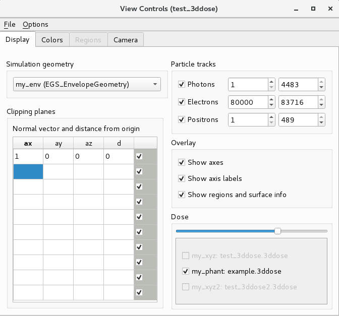
The egs_view display tab
The geometry currently being viewed is selected in the Simulation geometry section. This defaults to the simulation geometry specified in the input file. Clipping planes allow the user to view the internal structure of a geometry. For clipping planes, ax, ay and az define the unit normal to a planar surface. The surface can then be offset from the origin by setting the distance d [cm]. After typing in the 4 parameters, hit Enter to apply the clipping plane, or click away. Use the checkbox to the right of each clipping plane to toggle them on and off.
Particle tracks can be loaded in the viewer, if the simulation was configured to produce a ptracks file (using EGS_TrackScoring). One way to load the tracks is to launch egs_view with the ptracks file as an additional input. For example,
egs_view yourInput.egsinp yourInput.ptracks
Alternatively, load the ptracks file using File->Open tracks.... The range of tracks to view can be limited using the two input boxes next to each particle type. Note that you can also load previously saved settings from the command line by also listing the .egsview file, before or after the .ptracks file.
The dose, if scored to a 3ddose file, can be loaded using File->Open dose.... If a dose scoring ausgab object (EGS_DoseScoring) that is configured to produce a 3ddose file exists in the input file, then the 3ddose file will be automatically loaded and populate the list in the Dose section. The transparency of the dose is adjusted with the slider. If a 3ddose file is listed but disabled (or "grayed out"), this means that the 3ddose file dimensions did not match an EGS_XYZGeometry in the input file.
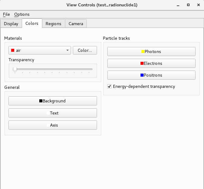
The egs_view colors tab
Various colors in the viewer can be controlled on this tab. Most importantly, material transparencies can be adjusted. Select the material of interest, set its color with the Color button, and set its transparency with the slider.
Setting the other view colors should be intuitive. The particle tracks also have a checkbox to toggle energy-dependent transparency. Enabled by default, this option allows the transparency of track lines to be adjusted depending on the energy of the particle. Particles with the highest energy will not be transparent at all, and the lowest energy particles will be the most transparent.
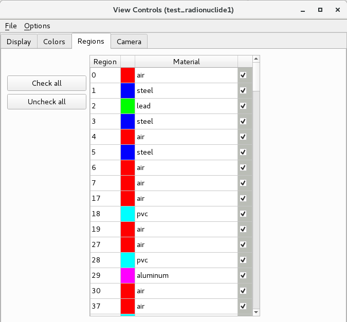
The egs_view regions tab
The Regions tab allows the user to enable or disable the display of specific regions in the geometry. It does not actually remove the region from the geometry, so it can still be found by hovering the mouse. Rather, it sets the transparency of the region to 0. It also lists the material and color of every region. Of course, for complex geometries this list would be prohibitively long and affect the performance of the application, so the tab is disabled if greater than 1000 regions are in the geometry.
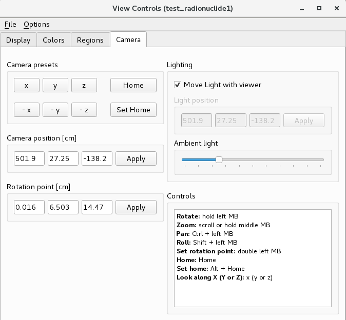
The egs_view camera tab
The Camera tab allows the user to control the camera position. A few camera presets are provided to look along each axis. To set a default view, position the camera as you like and click the Set Home button.
An alternative way to control the view is through directly setting the Camera position. This sets where you are looking from, in the coordinates of the geometry. However, the egs_view has a limitation that the Rotation point must reside within the geometry volume, and a constant distance between the camera position and the rotation point is automatically maintained when you change either parameter. If the new (automatic) rotation point falls outside the geometry, then the change fails to be applied and the camera position is reset to its last setting. Similarly, the user cannot directly set the rotation point itself outside the geometry.
To easily set the rotation point, double click on any surface in the geometry. The new rotation point will be set at that position.
Take note of the controls listed in the Controls section!
Example geometries
In the directory $HEN_HOUSE/egs++/geometry/examples there are several example input files specifying geometries for the egspp geometry package. They are provided with the hope that they will help the user to understand the concepts and learn the syntax of the geometry package. Here is a brief description of the examples and screen shots for some of them:
- The file
hemisphere.geomdefines a hemisphere using an N-dimensional geometry made of a set of spheres and a set of planes. - The file
pyramid.geomdefines a pyramid with an irregular base that is truncated at the two ends with a set of planes within an N-dimensional geometry. - The file
rz.geomdefines a RZ-geometry using an N-dimensional geometry made of a set of cylinders and a set of planes. The geometry defined is the same as in thecavrznrc_template.egsinpfile for the CAVRZnrc application (a simple pancake ionization chamber with graphite walls and air cavity). - The file
rz1.geomdefines the same geometry asrz.geombut now using an envelope geometry to inscribe a smaller cylinder into a larger one, where both cylinders are made using EGS_ConeStack objects. - The file
cones.geomdemonstrates the use of the EGS_ConeSet class. The user is encouraged to change theflagsetting to see how this changes the geometry.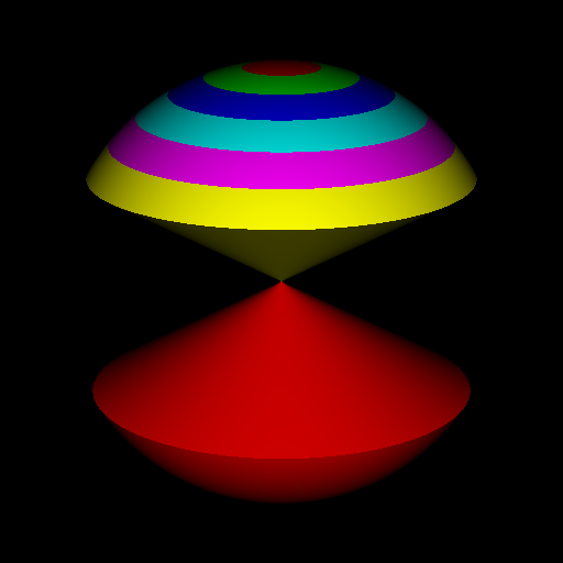 The cone geometry defined in cones.geom
 - The file
rz_phi.geomshows the use of I-planes to divide a cylinder into azimuthal segments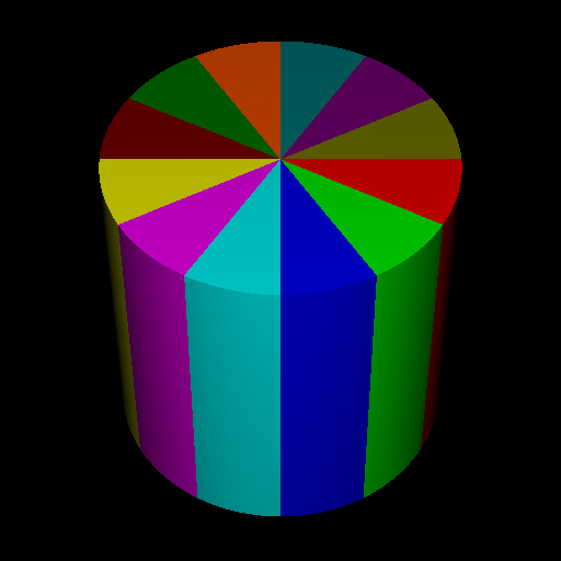 rz_phi.geom: using I-planes to divide a cylinder into segments
 - The file
xyz.geomdefines an XYZ-geometry filled with water and two inhomogeneities made of air and aluminum. mushroom.geomdefines a mushroom-like geometrical structure using a CD-geometry with a set of planes as a base and spheres and cylinders inscribed into the two regions defined by the planes.- The file
I6702.inpdefines a I model 6702 brachytherapy seed using a CD-geometry, sets of spheres for the rounded ends and an envelope containing the radioactive seeds for the middle portion
 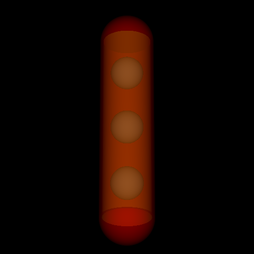 Model 6702 brachytherapy seed defined in I6702.inpThe two different views were generated using the transparency and clipping planes features of the geometry viewer.
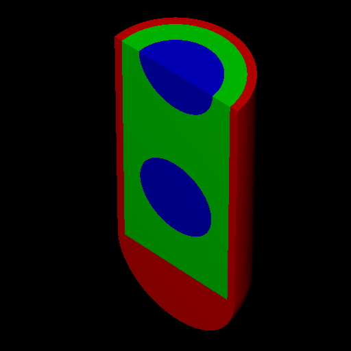 Model 6702 brachytherapy seed defined in I6702.inp
 - The file
rounded_ionchamber.geomdefines an ionization chamber geometry that has rounded ends using a CD-geometry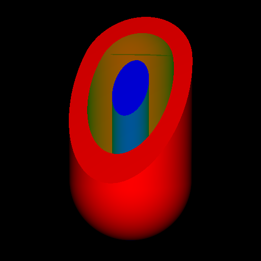 An ionization chamber with rounded ends defined in rounded_ionchamber.geom
 - The file
chambers_in_box.geomtakes the ion chamber described inrounded_ionchamber.geomand inscribes it, together with two transformed replicas, into a box of water using an envelope geometry (see the title page). - The files
seeds_in_xyz.geomandseeds_in_xyz1.geomdefine an XYZ-geometry containing 12 replicas of the brachytherapy seed specified inI6702.inp. The difference between the two is that in the one case the XYZ-geometry is used as the envelope in an envelope geometry whereas in the other case the XYZ-geometry is used as the base geometry of a CD-geometry. The user will quickly notice that the CD-geometry approach is substantially more efficient when trying to view these geometries with the geometry viewer. - The file
car.geomshows how to put together a car from simpler structures (EGS_ConeStack objects are used for the axis and wheels, boxes for the car body) using a union.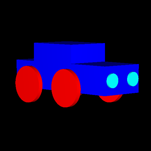 A car geometry defined in car.png
 - The file
photon_linac.geomshows how one can quickly put together a geometry model of the treatment head of a medical linear accelerator. The geometry defined in this file is identical to the 16 MV photon example that comes with the BEAMnrc distribution (except that the monitor chamber is not included).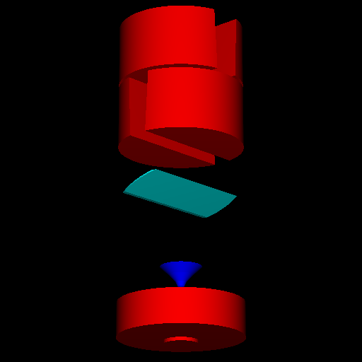 A Linac geometry defined in photon_linac.geom
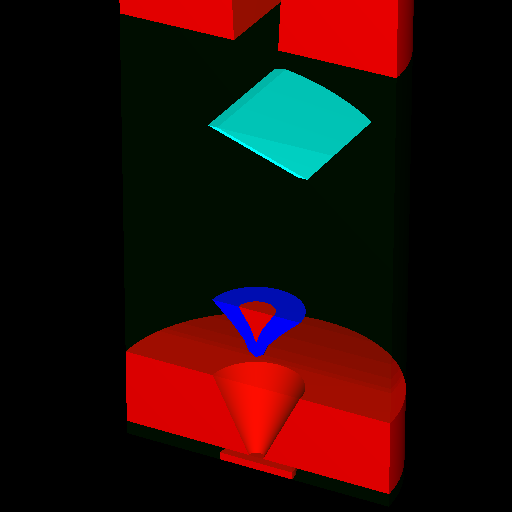 A different view of the geometry defined in photon_linac.geom
Note that all figures shown in this section were generated with the egspp geometry viewer. A more detailed description of the example geometries can be found here.
Macro Definition Documentation
◆ EGS_GLIB_
| #define EGS_GLIB_ |
egs_glib is a shim to be used in conjunction with the EGS Input include file directive for creating geometries defined in external files.
This is useful when you have a geometry defined in an external file:
 # your egsinp/geom file
:start geometry definition:

    :start geometry:
        library = egs_glib
        name = my_external_geom
        include file = /path/to/some/external/geom
    :stop geometry:

    :start geometry:
        library = egs_ndgeometry
        type = EGS_XYZGeometry
        name = my_base_geom
        x-planes =  -10 -5 0 5 10
        y-planes =  -10 -5 0 5 10
        z-planes =  -10 -5 0 5 10

        :start media input:
            media = WATER
        :stop media input:

    :stop geometry:

    :start geometry:
        library = egs_genvelope
        name = my_envelope_geom
        base geometry = my_base_geom
        inscribed geometries = my_external_geom
    :stop geometry:

    simulation geometry = my_envelope_geom

:stop geometry definition:
and then in your external file you would have something like:
 #The external geom (/path/to/some/external/geom)
:start geometry definition:

    :start geometry:
        library   = egs_spheres
        midpoint  = 0 0 0
        radii     = 4
        name      = the_sphere
        :start media input:
            media = medium1
        :stop media input:
    :stop geometry:

    simulation geometry = the_sphere

:stop geometry definition:
The above two definitions would result in a geometry equivalent to:
:start geometry definition:

    :start geometry:
        library   = egs_spheres
        midpoint  = 0 0 0
        radii     = 4
        name      = the_sphere
        :start media input:
            media = medium1
        :stop media input:
    :stop geometry:

    :start geometry:
        library = egs_ndgeometry
        type = XYZGeometry
        name = my_base_geom
        x-planes =  -10 5 0 5 10
        y-planes =  -10 5 0 5 10
        z-planes =  -10 5 0 5 10
    :stop geometry:

    :start geometry:
        library = egs_genvelope
        name = my_envelope_geom
        base geometry = my_base_geom
        inscribed geometries =  the_sphere
    :stop geometry:

    simulation geometry = my_envelope_geom

:stop geometry definition:
Examples
Examples of using the glib library are available in the glib.geom and seeds_in_xyz_aenv.geom files.
Definition at line 169 of file egs_glib.h.